Low Stable-Rank Structure in LoRA-DPO Adapters on Pythia 70M–1B: Empirical Scaling and Formal Invariants

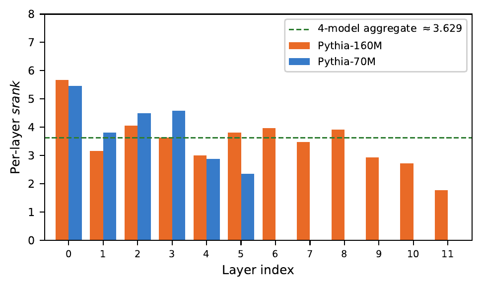
Debanjan Basu · 2026 · Pythia 70M–1B · code & data

We made the model four times wider. The adapter stable rank stayed at ≈3.6 — under this recipe, on this dataset.

Fine-tune a language model with LoRA under Direct Preference Optimization (LoRA-DPO) and the adapter concentrates in roughly 3–4 effective directions — across Pythia 70M–1B, trained on hh-rlhf with one fixed LoRA configuration (r=128, α=256, 800 steps). We call this width-stable low-rank structure under fixed recipe. Across the four scale points, a constant fits the stable-rank data better than either sub-linear decay we tested (RMS residual 0.289 vs. 0.431 for $c/d^{1/3}$ and 0.682 for $c/\sqrt{d}$) — but four points cannot distinguish a true constant from a mild monotone decay, and we have not varied the dataset or LoRA configuration to isolate causes.

Each dot is one model. Hover for exact values. The dashed line is the empirical floor at srank ≈ 3.6. LoRA's hard rank cap here is r = 128; the trained adapters sit ~32× below it.

3.6

average stable rank
across all models

4×

width increase,
srank floor unchanged

3–5×

above-chance subspace
alignment (γ signal)

Background

What does “stable rank 3.6” mean?

A LoRA adapter is a matrix — a grid of numbers that shifts a weight in the model. That matrix can be “wide” (spread across many directions in space) or “narrow” (concentrated in just a few). Stable rank measures this width: a value of 3.6 means the adapter’s energy is effectively spread across ~3–4 directions, even though the matrix formally has 128 dimensions.

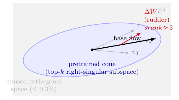
Think of a ship’s rudder. The ship is enormous. The rudder is tiny. But the rudder has one job — deflect the flow — and it does that job in a small number of geometric directions. Our finding: at every scale we measured, DPO used a “rudder” of about 3–4 directions, however large the ship. We measured four scales under one recipe; the analogy is a mnemonic, not a mechanism.

The surprising part: we expected larger models to learn richer, higher-dimensional alignment geometry. Under this fixed recipe and dataset, they don't. A 1B-parameter model uses the same number of effective directions as a 70M-parameter model fine-tuned on the same data. Whether retraining with different (r, α) or a different dataset would change this remains an open empirical question.

Formally: $\text{srank}(M) = |M|_F^2\, /\, |M|_2^2$. The numerator is total energy (sum of all squared singular values). The denominator is the energy in the single largest direction. The ratio tells you how many directions carry the energy. If all energy is in one direction, srank = 1. If energy is spread equally across 128 directions, srank = 128.

Crucially, srank is invariant to scaling: multiplying the matrix by any nonzero scalar leaves it unchanged. This matters for LoRA, where the $\alpha$ hyperparameter scales the adapter. We prove this formally in Lean 4 (stableRank_smul_invariant). So the srank ≈ 3.6 we measure cannot be a rescaling artifact of our α setting. The theorem covers post-hoc rescaling of a fixed learned matrix only — it says nothing about what training under a different α would converge to.

Key Finding

DPO and CLM concentrate in overlapping directions

Here is the second result. Training on preference data (DPO) vs. plain language modelling (CLM) produces different adapters — but the top singular vectors of each overlap the base weights’ top right-singular subspace at 3–5× the chance rate. We call this the γ-rudder signal. The objectives are not identical: at 1B, CLM overlaps more than DPO (4.08× vs. 3.36×, seed-averaged) — a measurable geometric cost of contrastive preference routing on this dataset.

The chart below shows, for each layer of a 1B-parameter model, how much DPO and CLM agree on the important directions. A value of 3× means their top-5 singular vectors share 3× more subspace than the analytic Haar-random expectation — the closed-form baseline E[overlap] = k/d for two uniformly-random k-frames in R^d (not a sampled approximation; exact for any finite d).

Four traces: DPO and CLM at two independent seeds (42 and 117). Independent data draws — yet the curves track closely. The signal is not a seed artifact.

The alignment is not confined to one part of the model. It appears in all four LoRA target modules — weakest in the attention output projection (≈2× above chance), strongest in the MLP projections.

What this means: on hh-rlhf, both objectives' top subspaces overlap the base weights' top right-singular subspace above the analytic Haar-random baseline (E[bonus] = 1 exactly; E[p(k)] = k/d). Read this carefully: the enrichment is angular, not bulk. Only ~0.8–1.1% of the adapters' absolute Frobenius mass lies inside the top-5 base cone at 1B — the rudder is a statistical bias toward existing flow, not literal confinement. And a behavioral cross-check (T1.2, Fig G) shows higher γ does not predict larger reward margin; the correlation is negative. Geometric structure and behavioral outcome are decoupled on this dataset.

What we ruled out

Three explanations that didn’t survive

Before concluding the srank floor is real, we tried to explain it away with three targeted alternatives. All three failed, though they do not exhaust the space of possible confounds.

Attempt 1: maybe it’s just the biases. If LayerNorm gain vectors (the LayerNorm γ parameters — unrelated to the γ-rudder signal above) span the adapter’s subspace, then the geometry would be trivially determined by initialization — not preference learning. We tested this by projecting each DPO adapter onto the LayerNorm gain subspace. Result: 99.97% of the energy lies outside it. This rules out the LayerNorm-gain subspace as an explanation. It does NOT rule out a broader class of pretrained-anisotropy explanations (weight curvature, weight-tying, token-frequency bias, optimizer-induced anisotropy).

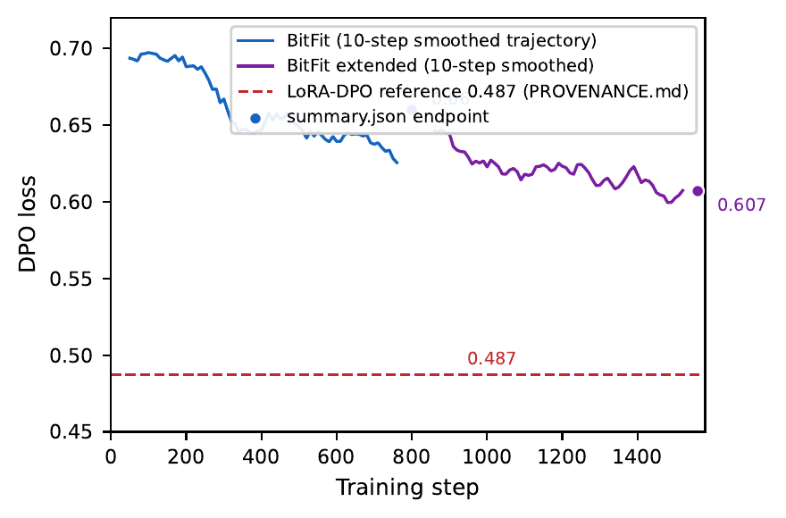
Attempt 2: maybe bias-only fine-tuning reproduces it. BitFit trains only bias parameters — no weight matrices at all. If BitFit-DPO matched the LoRA-DPO loss reduction, the geometric signal would be “gauge-accessible” (reachable without learning any subspace). It doesn’t: by step 800, BitFit captures 16% of the LoRA loss reduction, and an extension to 1560 steps still leaves it above the LoRA endpoint (0.607 final, 0.567 minimum, vs. 0.487).

BitFit vs LoRA loss trajectories — BitFit-DPO (orange) reduces loss to **0.660** at step 800, well above the LoRA-DPO endpoint of **0.487**. The gap means only ≈16% of the LoRA loss reduction is reachable through biases at matched steps — consistent with LoRA learning geometry that biases alone cannot replicate in this setting. BitFit does keep improving with more steps (0.607 at step 1560), so the gap is a strong trend at this budget, not a proven asymptote.

Attempt 3: maybe depth carries structure. If DPO adapters form a “quasiparticle” — a correlated pattern that travels across layers — we’d expect the layer-depth correlator $C(L, L+k)$ to decay with $k$. Measured at Pythia-410M, it doesn’t: the correlator stays near Pearson ≈ 0.97 regardless of depth gap. A flat correlator is inconsistent with the quasiparticle picture; it does not rule out depth structure that this particular statistic cannot see.

Formal grounding

Ruling out a measurement artifact from α or r

One might worry: maybe we’re measuring an artifact of hyperparameter choice. If we change the LoRA scaling $\alpha$, does srank change?

We prove it doesn’t — formally, in Lean 4:

stableRank_smul_invariant — scaling a fixed learned matrix by any $\lambda \neq 0$ leaves srank unchanged
rsLoraUpdate_frob_bounded — Frobenius energy obeys $|\Delta W|_F^2 \leq \alpha^2 c$, while srank is invariant to the scalar

The proofs use Mathlib’s linear algebra library and are machine-checked — a guarantee that applies to the 13 fully proven theorems; partial and deferred items are disclosed on the status page and none are cited as proved results. This rules out a trivial measurement artifact: the observed srank ≈ 3.6 is not an artifact of our α setting. Important caveat: the theorems concern post-hoc rescaling of a fixed learned matrix. They do NOT imply that retraining with different (α, r) would converge to the same geometry — that is an open empirical question.

Conceptual schematic: the lazy rudder — The pretrained model occupies a large subspace (blue ellipse). The DPO adapter (red arrow) is concentrated in ~3–4 directions — a small rudder on a large ship. The α hyperparameter controls the length of the arrow; the formal invariant shows direction is unchanged by α scaling of a fixed matrix.

See the Lean proof status →

For the curious

How the experiments work

Models. Pythia 70M, 160M, 410M, 1B (EleutherAI). Pre-trained, no instruction tuning.

LoRA. $r=128$, $\alpha=256$. Targets: query_key_value, dense, dense_h_to_4h, dense_4h_to_h. 800 training steps, LR=5e-6, cosine schedule, fp16.

Data. Anthropic/hh-rlhf, 2000 samples. DPO uses preference pairs. CLM uses chosen responses only (no rejection signal).

Reproducibility. All adapter checkpoints are mirrored at d3banjan/lazy-rudder-checkpoints (~1.9 GB). Every figure regenerates from make analysis && make paper. Per-checkpoint hashes, training configs, and seeds are recorded in PROVENANCE.md.

Per-layer srank for 70M and 160M — Per-layer stable rank for Pythia-70M and Pythia-160M. Smaller models put more dimensions into early layers than late ones (70M: early-quartile srank 5.5 vs. late 2.4); the asymmetry shrinks with scale and is gone at 1B (3.22 vs. 3.21). We report this as a layer-depth pattern under this recipe, not a scaling law.

Reviewer M9 response

Geometry–behavior decoupling (T1.2)

We measured reward margin and KL-to-base on 495 clean held-out Anthropic/hh-rlhf test examples for all five DPO checkpoints (70M, 160M, 410M, 1B×2 seeds), β=0.1, fp16.

Reward margin = β · [log π_θ(y_win

x)/π_ref(y_win

x) − log π_θ(y_los

x)/π_ref(y_los

x)]. KL-to-base = mean per-token log-ratio of DPO vs base on chosen response (teacher-forced; negative = DPO keeps probability close to or below base, consistent with β-regularization).

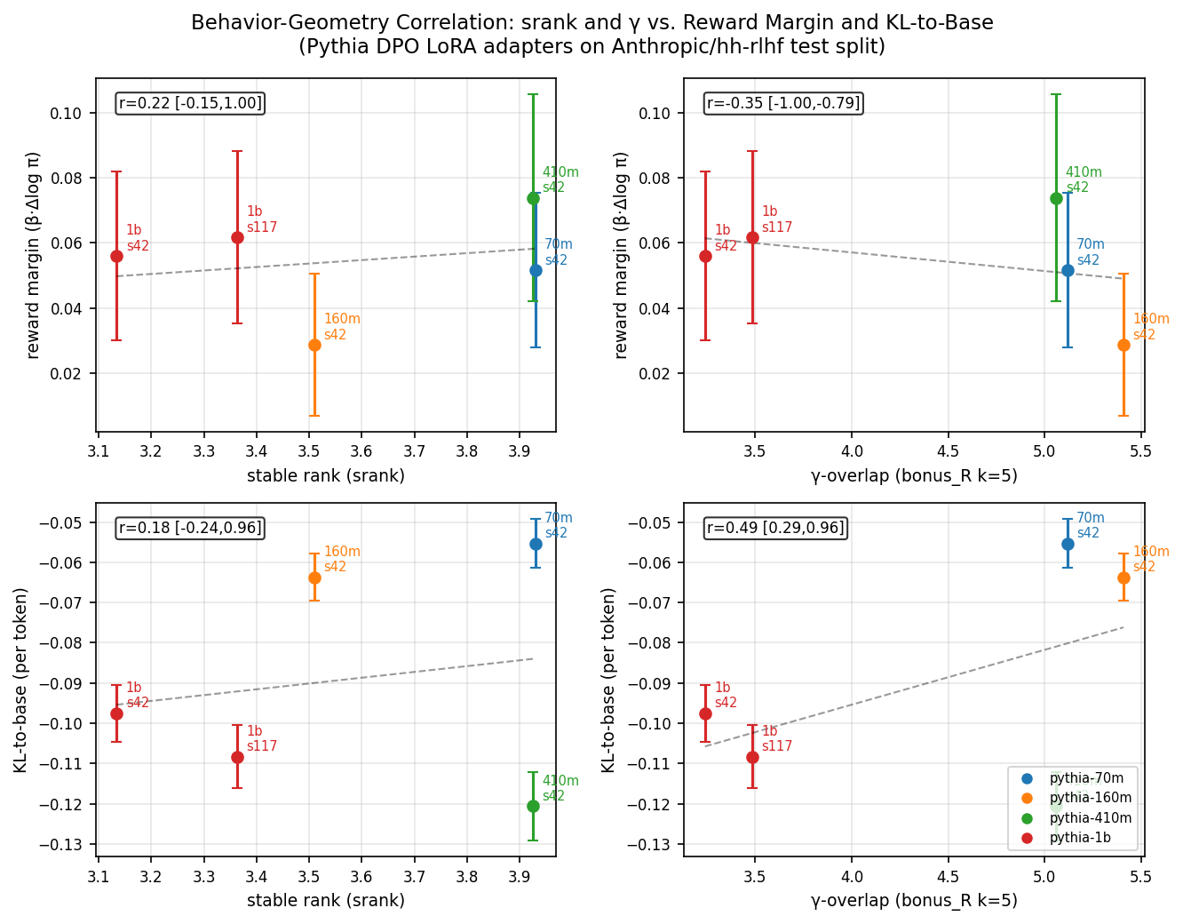
Geometry-behavior decoupling scatter grid — **Fig G — decoupling evidence.** 2×2 scatter: (srank, γ) × (reward margin, KL-to-base). Each point is one DPO checkpoint. Error bars = ±1 SE over 495 examples. Pearson r with 95% bootstrap CI in each panel. n=5; all CIs are wide and one pins at ±1 — treat as suggestive, not definitive. The γ–reward-margin Pearson is −0.35 (Spearman −0.60): higher subspace overlap predicts *lower* reward margin, opposite to the benign-steering prior. The γ–KL-to-base Pearson is +0.49: higher overlap co-occurs with greater divergence from base. The srank–reward-margin Pearson is near zero. T2.1 and T1.3 are the adjudicating experiments.

Primary finding: structural geometry and behavioral outcome are decoupled. Geometric alignment (γ) does not predict reward; it predicts KL drift. Tighter overlap with pretrained right-subspaces correlates with more divergence from the base distribution and lower reward margin — not efficient alignment. Stable rank (srank) is uncorrelated with reward margin across this scale range: it measures the rigid geometric constraint under which learning is forced to happen (the width of the pipe), not how successful that learning turns out to be. Adapters with r=128, α=256 on hh-rlhf converge to srank ≈ 3.6 regardless of model size; reward margin varies independently. This decoupling — not a confirmation of benign steering — is the paper’s primary empirical result.

Caveat. n=5 checkpoints; bootstrap CIs are wide and one pins at ±1. The most parsimonious reading of the current data is decoupling, but confirmation requires T2.1 (non-Pythia replication) and T1.3 (additional seeds).

Open question

Does the srank floor persist, or is it a transient early-training artefact?

Reviewer M7 asked whether the observed srank ≈ 3–4 at step 800 reflects convergence or just an early-training lazy regime. The right test is a srank-vs-training-step trajectory for each model size.

[Pending] srank vs training step — **[Pending data]** This plot will show stable rank vs. training step for Pythia 70M, 160M, 410M, and 1B (LoRA-DPO, r=128). A plateau in the last 30–50% of training would rebut the transient-regime critique. Currently a placeholder — no intermediate LoRA checkpoints were saved during the original training runs. Pending re-training with `save_steps ≤ 100` or a SrankCallback. See `scripts/generate_fig_F.py` for the data schema.

What we know now. The loss curve (logged at 10-step intervals in trainer_state.json) decreases monotonically through step 800 with no plateau, suggesting training was active throughout. The srank floor is consistent across DPO and CLM objectives and across two independent seeds at 1B scale — harder to explain as a transient coincidence. These are supportive signals but not a substitute for a trajectory plot. We flag this as a Tier-1 follow-up.

Citation

Cite this work

@misc{basu2026lazyrudder, title = {Low Stable-Rank Structure in {LoRA}-{DPO} Adapters on {Pythia} 70M--1B: Empirical Scaling and Formal Invariants}, author = {Basu, Debanjan}, year = {2026}, url = {https://github.com/d3banjan/lazy-rudder-paper} }

References. Hu et al. (2022) LoRA; Rafailov et al. (2023) DPO; Kalajdzievski (2023) RsLoRA; Biderman et al. (2023) Pythia; Lean 4 + Mathlib (The Mathlib Community, 2020).